Backtest: validation on historical data
![]()
This notebook contains the simple examples of time series validation using backtest module of ETNA library.
Table of Contents
[2]:
import pandas as pd
import matplotlib.pyplot as plt

from etna.datasets.tsdataset import TSDataset
from etna.metrics import MAE
from etna.metrics import MSE
from etna.metrics import SMAPE
from etna.pipeline import Pipeline
from etna.models import ProphetModel
from etna.analysis import plot_backtest
1. What is backtest and how it works
Backtest is a predictions and validation pipeline build on historical data to make a legitimate retrotest of your model.
How does it work?
When constructing a forecast using Models and further evaluating the prediction metrics, we measure the quality at one time interval, designated as test.
Backtest allows you to simulate how the model would work in the past:
selects a period of time in the past
builds a model using the selected interval as a training sample
predicts the value on the test interval and calculates metrics.
The image shows a plot of the backtest pipeline with n_folds = 3.
[3]:
img = plt.imread("./assets/backtest/backtest.jpg")
plt.figure(figsize=(15, 10))
plt.axis("off")
_ = plt.imshow(img)
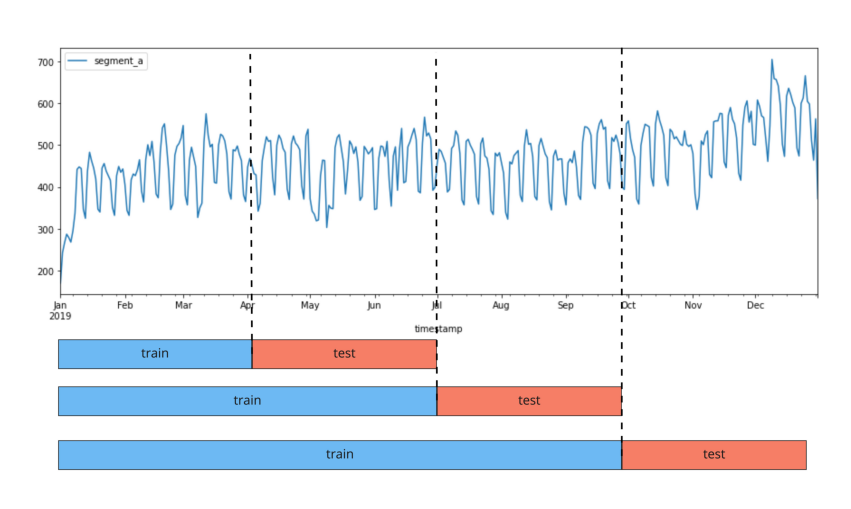
Below we will call a fold the train + test pair, for which training and forecasting is performed.
[4]:
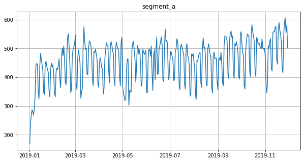
df = pd.read_csv("./data/example_dataset.csv")
df["timestamp"] = pd.to_datetime(df["timestamp"])
df = df.loc[df.segment == "segment_a"]
df.head()
[4]:
| timestamp | segment | target | |
|---|---|---|---|
| 0 | 2019-01-01 | segment_a | 170 |
| 1 | 2019-01-02 | segment_a | 243 |
| 2 | 2019-01-03 | segment_a | 267 |
| 3 | 2019-01-04 | segment_a | 287 |
| 4 | 2019-01-05 | segment_a | 279 |
Our library works with the special data structure TSDataset. So, before starting the EDA, we need to convert the classical DataFrame to TSDataset.
[5]:
df = TSDataset.to_dataset(df)
ts = TSDataset(df, freq="D")
2. How to run a validation
For an easy start let’s create a Prophet model
[7]:
horizon = 31  # Set the horizon for predictions
model = ProphetModel()  # Create a model
transforms = []  # A list of transforms -  we will not use any of them
Pipeline
Now let’s create an instance of Pipeline.
[8]:
pipeline = Pipeline(model=model, transforms=transforms, horizon=horizon)
We are going to run backtest method for it. As a result, three dataframes will be returned: * dataframe with metrics for each fold and each segment, * dataframe with predictions, * dataframe with information about folds.
[9]:
metrics_df, forecast_df, fold_info_df = pipeline.backtest(ts=ts, metrics=[MAE(), MSE(), SMAPE()])
[Parallel(n_jobs=1)]: Using backend SequentialBackend with 1 concurrent workers.
14:35:10 - cmdstanpy - INFO - Chain [1] start processing
14:35:10 - cmdstanpy - INFO - Chain [1] done processing
[Parallel(n_jobs=1)]: Done   1 out of   1 | elapsed:    1.1s remaining:    0.0s
14:35:11 - cmdstanpy - INFO - Chain [1] start processing
14:35:11 - cmdstanpy - INFO - Chain [1] done processing
[Parallel(n_jobs=1)]: Done   2 out of   2 | elapsed:    2.1s remaining:    0.0s
14:35:12 - cmdstanpy - INFO - Chain [1] start processing
14:35:12 - cmdstanpy - INFO - Chain [1] done processing
[Parallel(n_jobs=1)]: Done   3 out of   3 | elapsed:    3.0s remaining:    0.0s
14:35:13 - cmdstanpy - INFO - Chain [1] start processing
14:35:13 - cmdstanpy - INFO - Chain [1] done processing
[Parallel(n_jobs=1)]: Done   4 out of   4 | elapsed:    4.1s remaining:    0.0s
14:35:14 - cmdstanpy - INFO - Chain [1] start processing
14:35:14 - cmdstanpy - INFO - Chain [1] done processing
[Parallel(n_jobs=1)]: Done   5 out of   5 | elapsed:    5.1s remaining:    0.0s
[Parallel(n_jobs=1)]: Done   5 out of   5 | elapsed:    5.1s finished
[10]:
metrics_df.head()
[10]:
| segment | MAE | MSE | SMAPE | fold_number | |
|---|---|---|---|---|---|
| 0 | segment_a | 18.851344 | 595.763719 | 4.372066 | 0 |
| 0 | segment_a | 21.026910 | 673.249070 | 4.842875 | 1 |
| 0 | segment_a | 30.107632 | 1315.679297 | 6.302994 | 2 |
| 0 | segment_a | 36.204963 | 2021.144120 | 7.470983 | 3 |
| 0 | segment_a | 32.003925 | 1872.618930 | 6.470948 | 4 |
[11]:
forecast_df.head()
[11]:
| segment | segment_a | |
|---|---|---|
| feature | fold_number | target |
| timestamp | ||
| 2019-06-29 | 0 | 395.286255 |
| 2019-06-30 | 0 | 386.204016 |
| 2019-07-01 | 0 | 493.164874 |
| 2019-07-02 | 0 | 509.586239 |
| 2019-07-03 | 0 | 497.749328 |
[12]:
fold_info_df.head()
[12]:
| train_start_time | train_end_time | test_start_time | test_end_time | fold_number | |
|---|---|---|---|---|---|
| 0 | 2019-01-01 | 2019-06-28 | 2019-06-29 | 2019-07-29 | 0 |
| 0 | 2019-01-01 | 2019-07-29 | 2019-07-30 | 2019-08-29 | 1 |
| 0 | 2019-01-01 | 2019-08-29 | 2019-08-30 | 2019-09-29 | 2 |
| 0 | 2019-01-01 | 2019-09-29 | 2019-09-30 | 2019-10-30 | 3 |
| 0 | 2019-01-01 | 2019-10-30 | 2019-10-31 | 2019-11-30 | 4 |
You can additionally get the metrics averaged over folds:
[13]:
metrics_df, forecast_df, fold_info_df = pipeline.backtest(
    ts=ts, metrics=[MAE(), MSE(), SMAPE()], aggregate_metrics=True
)
[Parallel(n_jobs=1)]: Using backend SequentialBackend with 1 concurrent workers.
14:35:20 - cmdstanpy - INFO - Chain [1] start processing
14:35:20 - cmdstanpy - INFO - Chain [1] done processing
[Parallel(n_jobs=1)]: Done   1 out of   1 | elapsed:    1.0s remaining:    0.0s
14:35:21 - cmdstanpy - INFO - Chain [1] start processing
14:35:21 - cmdstanpy - INFO - Chain [1] done processing
[Parallel(n_jobs=1)]: Done   2 out of   2 | elapsed:    1.9s remaining:    0.0s
14:35:22 - cmdstanpy - INFO - Chain [1] start processing
14:35:22 - cmdstanpy - INFO - Chain [1] done processing
[Parallel(n_jobs=1)]: Done   3 out of   3 | elapsed:    2.9s remaining:    0.0s
14:35:23 - cmdstanpy - INFO - Chain [1] start processing
14:35:23 - cmdstanpy - INFO - Chain [1] done processing
[Parallel(n_jobs=1)]: Done   4 out of   4 | elapsed:    4.0s remaining:    0.0s
14:35:24 - cmdstanpy - INFO - Chain [1] start processing
14:35:24 - cmdstanpy - INFO - Chain [1] done processing
[Parallel(n_jobs=1)]: Done   5 out of   5 | elapsed:    5.0s remaining:    0.0s
[Parallel(n_jobs=1)]: Done   5 out of   5 | elapsed:    5.0s finished
[14]:
metrics_df.head()
[14]:
| segment | MAE | MSE | SMAPE | |
|---|---|---|---|---|
| 0 | segment_a | 27.638955 | 1295.691027 | 5.891973 |
[15]:
forecast_df.head()
[15]:
| segment | segment_a | |
|---|---|---|
| feature | fold_number | target |
| timestamp | ||
| 2019-06-29 | 0 | 395.286255 |
| 2019-06-30 | 0 | 386.204016 |
| 2019-07-01 | 0 | 493.164874 |
| 2019-07-02 | 0 | 509.586239 |
| 2019-07-03 | 0 | 497.749328 |
[16]:
fold_info_df.head()
[16]:
| train_start_time | train_end_time | test_start_time | test_end_time | fold_number | |
|---|---|---|---|---|---|
| 0 | 2019-01-01 | 2019-06-28 | 2019-06-29 | 2019-07-29 | 0 |
| 0 | 2019-01-01 | 2019-07-29 | 2019-07-30 | 2019-08-29 | 1 |
| 0 | 2019-01-01 | 2019-08-29 | 2019-08-30 | 2019-09-29 | 2 |
| 0 | 2019-01-01 | 2019-09-29 | 2019-09-30 | 2019-10-30 | 3 |
| 0 | 2019-01-01 | 2019-10-30 | 2019-10-31 | 2019-11-30 | 4 |
3. Backtest with fold masks
You can use your backtest strategies using FoldMask. In order to make a FoldMask, you need to specify first_train_timestamp, last_train_timestamp, target_timestamps. Then you need to pass a list of masks as the n_folds parameter to the pipeline.backtest.
Consider 3 strategies similar to SlidingWindowSplitter, ExpandingWindowSplitter and SingleWindowSplitter from sktime.
ExpandingWindowSplitter
For this backtest strategy you can use our backtest with mode="expand".
[17]:
metrics_df, _, _ = pipeline.backtest(ts=ts, metrics=[MAE(), MSE(), SMAPE()], n_folds=3, mode="expand")
[Parallel(n_jobs=1)]: Using backend SequentialBackend with 1 concurrent workers.
14:35:30 - cmdstanpy - INFO - Chain [1] start processing
14:35:30 - cmdstanpy - INFO - Chain [1] done processing
[Parallel(n_jobs=1)]: Done   1 out of   1 | elapsed:    1.0s remaining:    0.0s
14:35:31 - cmdstanpy - INFO - Chain [1] start processing
14:35:31 - cmdstanpy - INFO - Chain [1] done processing
[Parallel(n_jobs=1)]: Done   2 out of   2 | elapsed:    2.0s remaining:    0.0s
14:35:32 - cmdstanpy - INFO - Chain [1] start processing
14:35:32 - cmdstanpy - INFO - Chain [1] done processing
[Parallel(n_jobs=1)]: Done   3 out of   3 | elapsed:    3.0s remaining:    0.0s
[Parallel(n_jobs=1)]: Done   3 out of   3 | elapsed:    3.0s finished
[18]:
metrics_df
[18]:
| segment | MAE | MSE | SMAPE | fold_number | |
|---|---|---|---|---|---|
| 0 | segment_a | 30.107632 | 1315.679297 | 6.302994 | 0 |
| 0 | segment_a | 36.204963 | 2021.144120 | 7.470983 | 1 |
| 0 | segment_a | 32.003925 | 1872.618930 | 6.470948 | 2 |
SingleWindowSplitter
For this backtest strategy you can use our backtest with parameter n_folds=1 or if you need specific window from your dataset you can create a mask with FoldMask.
[19]:
from etna.pipeline import FoldMask
import numpy as np
[20]:
# 1 Without mask

metrics_df, _, _ = pipeline.backtest(ts=ts, metrics=[MAE(), MSE(), SMAPE()], n_folds=1)
metrics_df
[Parallel(n_jobs=1)]: Using backend SequentialBackend with 1 concurrent workers.
14:35:33 - cmdstanpy - INFO - Chain [1] start processing
14:35:33 - cmdstanpy - INFO - Chain [1] done processing
[Parallel(n_jobs=1)]: Done   1 out of   1 | elapsed:    1.0s remaining:    0.0s
[Parallel(n_jobs=1)]: Done   1 out of   1 | elapsed:    1.0s finished
[20]:
| segment | MAE | MSE | SMAPE | fold_number | |
|---|---|---|---|---|---|
| 0 | segment_a | 32.003925 | 1872.61893 | 6.470948 | 0 |
[21]:
# 2 With specific mask
window_size = 85
first_train_timestamp = ts.index.min() + np.timedelta64(100, "D")
last_train_timestamp = first_train_timestamp + np.timedelta64(window_size, "D")
target_timestamps = pd.date_range(start=last_train_timestamp + np.timedelta64(1, "D"), periods=horizon)
mask = FoldMask(
    first_train_timestamp=first_train_timestamp,
    last_train_timestamp=last_train_timestamp,
    target_timestamps=target_timestamps,
)
[22]:
# 1 Without mask

metrics_df, _, _ = pipeline.backtest(ts=ts, metrics=[MAE(), MSE(), SMAPE()], n_folds=[mask])
metrics_df
[Parallel(n_jobs=1)]: Using backend SequentialBackend with 1 concurrent workers.
14:35:34 - cmdstanpy - INFO - Chain [1] start processing
14:35:35 - cmdstanpy - INFO - Chain [1] done processing
[Parallel(n_jobs=1)]: Done   1 out of   1 | elapsed:    1.1s remaining:    0.0s
[Parallel(n_jobs=1)]: Done   1 out of   1 | elapsed:    1.1s finished
[22]:
| segment | MAE | MSE | SMAPE | fold_number | |
|---|---|---|---|---|---|
| 0 | segment_a | 39.782294 | 2191.914485 | 9.056343 | 0 |
SlidingWindowSplitter
To implement this backtest strategy you need to create a list of fold masks with FoldMask.
[23]:
n_folds = 3
[24]:
def sliding_window_masks(window_size, n_folds):
    masks = []
    for n in range(n_folds):
        first_train_timestamp = ts.index.min() + np.timedelta64(100, "D") + np.timedelta64(n, "D")
        last_train_timestamp = first_train_timestamp + np.timedelta64(window_size, "D")
        target_timestamps = pd.date_range(start=last_train_timestamp + np.timedelta64(1, "D"), periods=horizon)
        mask = FoldMask(
            first_train_timestamp=first_train_timestamp,
            last_train_timestamp=last_train_timestamp,
            target_timestamps=target_timestamps,
        )
        masks.append(mask)
    return masks
[25]:
masks = sliding_window_masks(window_size=window_size, n_folds=n_folds)
metrics_df, _, _ = pipeline.backtest(ts=ts, metrics=[MAE(), MSE(), SMAPE()], n_folds=masks)
[Parallel(n_jobs=1)]: Using backend SequentialBackend with 1 concurrent workers.
14:35:36 - cmdstanpy - INFO - Chain [1] start processing
14:35:36 - cmdstanpy - INFO - Chain [1] done processing
[Parallel(n_jobs=1)]: Done   1 out of   1 | elapsed:    1.3s remaining:    0.0s
14:35:37 - cmdstanpy - INFO - Chain [1] start processing
14:35:37 - cmdstanpy - INFO - Chain [1] done processing
[Parallel(n_jobs=1)]: Done   2 out of   2 | elapsed:    2.4s remaining:    0.0s
14:35:38 - cmdstanpy - INFO - Chain [1] start processing
14:35:38 - cmdstanpy - INFO - Chain [1] done processing
[Parallel(n_jobs=1)]: Done   3 out of   3 | elapsed:    3.6s remaining:    0.0s
[Parallel(n_jobs=1)]: Done   3 out of   3 | elapsed:    3.6s finished
[26]:
metrics_df
[26]:
| segment | MAE | MSE | SMAPE | fold_number | |
|---|---|---|---|---|---|
| 0 | segment_a | 39.782294 | 2191.914485 | 9.056343 | 0 |
| 0 | segment_a | 40.293273 | 2287.327210 | 9.108208 | 1 |
| 0 | segment_a | 39.861473 | 2192.540812 | 9.010115 | 2 |
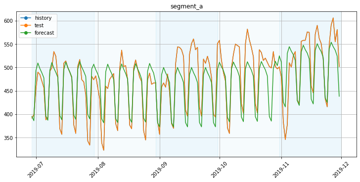
4. Validation visualisation
[27]:
plot_backtest(forecast_df, ts)
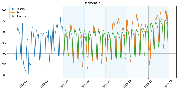
To visualize the train part, you can specify the history_len parameter.
[28]:
plot_backtest(forecast_df, ts, history_len=70)
5. Metrics visualization
In this section we will analyze the backtest results from the different point of views.
[29]:
from etna.analysis import (
    metric_per_segment_distribution_plot,
    plot_residuals,
    plot_metric_per_segment,
    prediction_actual_scatter_plot,
)
[30]:
df = pd.read_csv("./data/example_dataset.csv")
df["timestamp"] = pd.to_datetime(df["timestamp"])
df = TSDataset.to_dataset(df)
ts_all = TSDataset(df, freq="D")
[31]:
metrics_df, forecast_df, fold_info_df = pipeline.backtest(ts=ts_all, metrics=[MAE(), MSE(), SMAPE()])
[Parallel(n_jobs=1)]: Using backend SequentialBackend with 1 concurrent workers.
14:35:42 - cmdstanpy - INFO - Chain [1] start processing
14:35:42 - cmdstanpy - INFO - Chain [1] done processing
14:35:42 - cmdstanpy - INFO - Chain [1] start processing
14:35:42 - cmdstanpy - INFO - Chain [1] done processing
14:35:42 - cmdstanpy - INFO - Chain [1] start processing
14:35:42 - cmdstanpy - INFO - Chain [1] done processing
14:35:42 - cmdstanpy - INFO - Chain [1] start processing
14:35:42 - cmdstanpy - INFO - Chain [1] done processing
[Parallel(n_jobs=1)]: Done   1 out of   1 | elapsed:    3.8s remaining:    0.0s
14:35:46 - cmdstanpy - INFO - Chain [1] start processing
14:35:46 - cmdstanpy - INFO - Chain [1] done processing
14:35:46 - cmdstanpy - INFO - Chain [1] start processing
14:35:46 - cmdstanpy - INFO - Chain [1] done processing
14:35:46 - cmdstanpy - INFO - Chain [1] start processing
14:35:46 - cmdstanpy - INFO - Chain [1] done processing
14:35:46 - cmdstanpy - INFO - Chain [1] start processing
14:35:46 - cmdstanpy - INFO - Chain [1] done processing
[Parallel(n_jobs=1)]: Done   2 out of   2 | elapsed:    7.6s remaining:    0.0s
14:35:49 - cmdstanpy - INFO - Chain [1] start processing
14:35:50 - cmdstanpy - INFO - Chain [1] done processing
14:35:50 - cmdstanpy - INFO - Chain [1] start processing
14:35:50 - cmdstanpy - INFO - Chain [1] done processing
14:35:50 - cmdstanpy - INFO - Chain [1] start processing
14:35:50 - cmdstanpy - INFO - Chain [1] done processing
14:35:50 - cmdstanpy - INFO - Chain [1] start processing
14:35:50 - cmdstanpy - INFO - Chain [1] done processing
[Parallel(n_jobs=1)]: Done   3 out of   3 | elapsed:   11.4s remaining:    0.0s
14:35:53 - cmdstanpy - INFO - Chain [1] start processing
14:35:53 - cmdstanpy - INFO - Chain [1] done processing
14:35:53 - cmdstanpy - INFO - Chain [1] start processing
14:35:53 - cmdstanpy - INFO - Chain [1] done processing
14:35:53 - cmdstanpy - INFO - Chain [1] start processing
14:35:53 - cmdstanpy - INFO - Chain [1] done processing
14:35:53 - cmdstanpy - INFO - Chain [1] start processing
14:35:53 - cmdstanpy - INFO - Chain [1] done processing
[Parallel(n_jobs=1)]: Done   4 out of   4 | elapsed:   15.3s remaining:    0.0s
14:35:57 - cmdstanpy - INFO - Chain [1] start processing
14:35:57 - cmdstanpy - INFO - Chain [1] done processing
14:35:57 - cmdstanpy - INFO - Chain [1] start processing
14:35:57 - cmdstanpy - INFO - Chain [1] done processing
14:35:57 - cmdstanpy - INFO - Chain [1] start processing
14:35:57 - cmdstanpy - INFO - Chain [1] done processing
14:35:57 - cmdstanpy - INFO - Chain [1] start processing
14:35:57 - cmdstanpy - INFO - Chain [1] done processing
[Parallel(n_jobs=1)]: Done   5 out of   5 | elapsed:   19.1s remaining:    0.0s
[Parallel(n_jobs=1)]: Done   5 out of   5 | elapsed:   19.1s finished
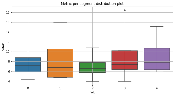
Let’s look at the distribution of the SMAPE metric by folds. You can set type_plot as box, violin or hist.
[32]:
metric_per_segment_distribution_plot(metrics_df=metrics_df, metric_name="SMAPE", plot_type="box")
Let’s look at the SMAPE metric by segments
[33]:
plot_metric_per_segment(metrics_df=metrics_df, metric_name="SMAPE", ascending=True)

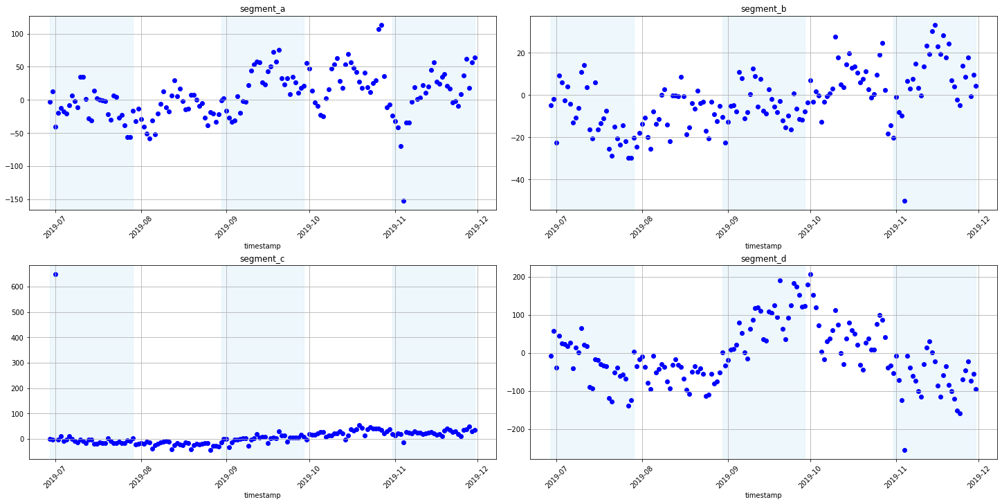
Now let’s look at the residuals of the model predictions from the backtest. Analysis of the residuals can help establish a dependency in the data that our model was not able to find. This way we can add features or improve the model or make sure that there is no dependency in the residuals. Also, you can visualize the residuals not only by timestamp but by any feature.
[34]:
plot_residuals(forecast_df=forecast_df, ts=ts_all)
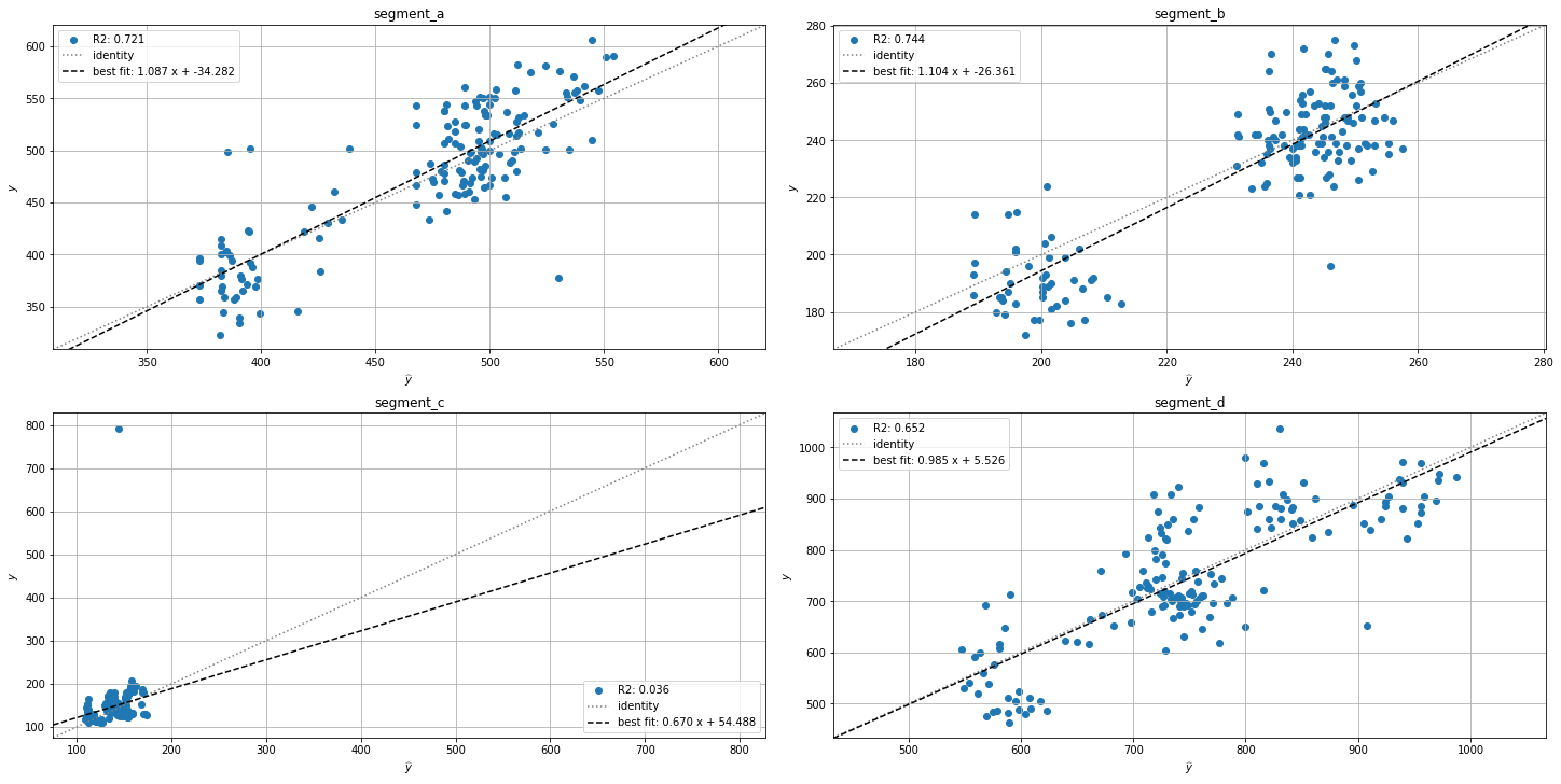
[35]:
prediction_actual_scatter_plot(forecast_df=forecast_df, ts=ts_all)
That’s all for this notebook. More features you can find in our documentation!