Clustering notebook
![]()
This notebook contains the simple examples of timeseries clustering using ETNA library.
Table of Contents
[1]:
import warnings

warnings.filterwarnings("ignore")
1. Generating dataset
In this notebook we will work with the toy dataset generated from Normal distribution. Timeseries are naturally separated into clusters based on the mean value.
[2]:
from etna.datasets import TSDataset
import pandas as pd
import numpy as np
[3]:
def gen_dataset():
    df = pd.DataFrame()
    for i in range(1, 5):
        date_range = pd.date_range("2020-01-01", "2020-05-01")
        for j, sigma in enumerate([0.1, 0.3, 0.5, 0.8]):
            tmp = pd.DataFrame({"timestamp": date_range})
            tmp["segment"] = f"{2*i}{j}"
            tmp["target"] = np.random.normal(2 * i, sigma, len(tmp))
            df = df.append(tmp, ignore_index=True)
    ts = TSDataset(df=TSDataset.to_dataset(df), freq="D")
    return ts
Let’s take a look at the dataset
[4]:
ts = gen_dataset()
ts.df.plot(figsize=(20, 10), legend=False);
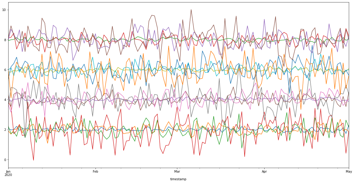
As you can see, there are about four clusters here. However, usually it is not obvious how to separate the timeseries into the clusters. Therefore, we might want to use clustering algorithms to help us.
2. Distance
In order to combine series into clusters, it is necessary to set the distance function on them. Distances implement the Distance interface and can be computed for two pd.Series indexed by timestamp.
In our library we provide implementation of Euclidean and DTW Distances
[5]:
from etna.clustering import EuclideanDistance, DTWDistance
[6]:
x1 = pd.Series(
    data=[0, 0, 1, 2, 3, 4, 5, 6, 7, 8],
    index=pd.date_range("2020-01-01", periods=10),
)
x2 = pd.Series(
    data=[0, 1, 2, 3, 4, 5, 6, 7, 8, 9],
    index=pd.date_range("2020-01-02", periods=10),
)
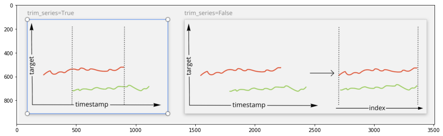
Distance calculation in the case of different timestamps can be performed in two modes: * trim_series = True - calculate the distance only over the common part of the series. Common part is defined based on the timestamp index.
[7]:
distance = EuclideanDistance(trim_series=True)
distance(x1, x2)  # Series are the same in the common part of the timestamps
[7]:
0.0
trim_series = False- calculate the distance over the whole series, ignoring the timestamp. The same as dropping the timestamp index and using the integer index as in the common array.
[8]:
distance = EuclideanDistance(trim_series=False)
distance(x1, x2)
[8]:
3.0
For better understanding, take a look at the visualization below.
[9]:
import matplotlib.pyplot as plt

_ = plt.subplots(figsize=(15, 10))
img = plt.imread("./assets/clustering/trim_series.jpg")
plt.imshow(img);
Let’s calculate different Distances with setting trim_series parameter to see the difference
[10]:
distances = pd.DataFrame()
distances["Euclidean"] = [
    EuclideanDistance(trim_series=True)(x1, x2),
    EuclideanDistance(trim_series=False)(x1, x2),
]
distances["DTW"] = [
    DTWDistance(trim_series=True)(x1, x2),
    DTWDistance(trim_series=False)(x1, x2),
]
distances["trim_series"] = [True, False]
distances.set_index("trim_series", inplace=True)
distances
[10]:
| Euclidean | DTW | |
|---|---|---|
| trim_series | ||
| True | 0.0 | 0.0 |
| False | 3.0 | 1.0 |
3. Clustering
Our library provides a class for so called hierarchical clustering, which has two built-in implementations for different Distances.
[11]:
from etna.clustering import EuclideanClustering
Hierarchical clustering consists of three stages: 1. Building a matrix of pairwise distances between series (build_distance_matrix) 2. Initializing the clustering algorithm (build_clustering_algo) 3. Training the clustering algorithm and predicting clusters (fit_predict)
In this section you will find the description of step by step clustering process.
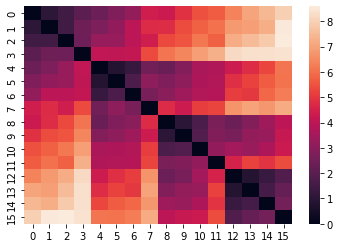
3.1 Build Distance Matrix
On the first step we need to build the so-called Distance matrix containing the pairwise distances between the timeseries in the dataset. Note, that this is the most time-consuming part of the clustering process, and it may take a long time to build a Distance matrix for a large dataset.
[12]:
import seaborn as sns
Distance matrix for the Euclidean distance
[13]:
model = EuclideanClustering()
model.build_distance_matrix(ts=ts)
sns.heatmap(model.distance_matrix.matrix);
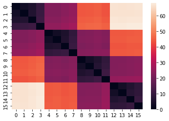
The Distance matrix is computed ones and saved in the instance of HierarchicalClustering. This makes it possible to change the clustering parameters without recalculating the Distance matrix.
3.2 Build Clustering algorithm
After computing the Distance matrix, you need to set the parameters to the clustering algorithm, such as: + n_clusters - number of clusters + linkage - rule for distance computation for new clusters
As the Distance matrix is build once, you can experiment with different parameters of the clustering algorithm without wasting time on its recomputation.
[14]:
model = EuclideanClustering()
model.build_distance_matrix(ts)
[15]:
model.build_clustering_algo(n_clusters=4, linkage="average")
3.3 Predict clusters
The final step of the clustering process is cluster prediction. As the output of the fit_predict you get the mapping for segment to cluster.
[16]:
segment2cluster = model.fit_predict()
segment2cluster
[16]:
{'20': 0,
 '21': 0,
 '22': 0,
 '23': 0,
 '40': 3,
 '41': 3,
 '42': 3,
 '43': 3,
 '60': 1,
 '61': 1,
 '62': 1,
 '63': 1,
 '80': 2,
 '81': 2,
 '82': 2,
 '83': 2}
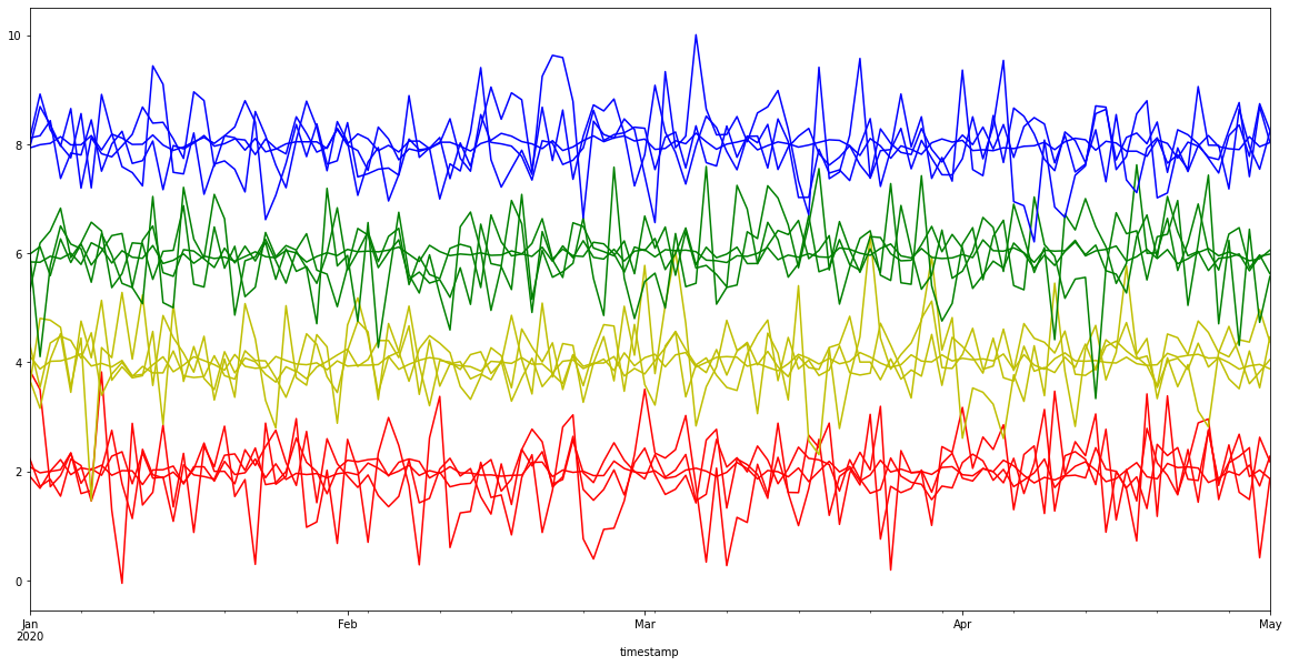
Let’s visualize the results
[17]:
colores = ["r", "g", "b", "y"]
color = [colores[i] for i in segment2cluster.values()]
ts.df.plot(figsize=(20, 10), color=color, legend=False);
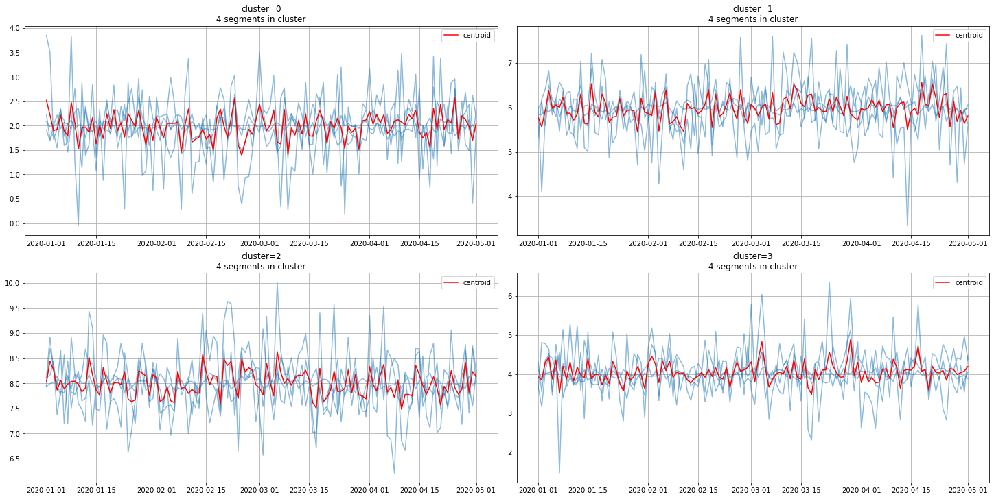
3.4 Get centroids
In addition, it is possible to get the clusters centroids, which are the typical member of the corresponding cluster.
[18]:
from etna.analysis import plot_clusters
[19]:
centroids = model.get_centroids()
centroids.head()
[19]:
| cluster | 0 | 1 | 2 | 3 |
|---|---|---|---|---|
| feature | target | target | target | target |
| timestamp | ||||
| 2020-01-01 | 2.519784 | 5.782033 | 8.025283 | 3.927396 |
| 2020-01-02 | 2.222438 | 5.562839 | 8.441052 | 3.845699 |
| 2020-01-03 | 1.894372 | 5.931193 | 8.268628 | 4.300714 |
| 2020-01-04 | 1.928784 | 6.374511 | 7.865045 | 4.419275 |
| 2020-01-05 | 2.209916 | 5.981512 | 8.059200 | 3.868911 |
Finally, we can plot clusters along with centroids for visual assessment
[20]:
plot_clusters(ts, segment2cluster, centroids)
4. Advanced: Custom Distance
In addition to the built-in Distances, you are able to implement your own Distance. The example below shows how to implement the Distance interface for custom Distance.
4.1 Custom Distance implementation
[21]:
from etna.clustering import Distance


class MyDistance(Distance):
    def __init__(self, trim_series: bool = False):
        super().__init__(trim_series=trim_series)

    def _compute_distance(self, x1: np.ndarray, x2: np.ndarray) -> float:
        """Compute distance between x1 and x2."""
        return np.max(np.abs(x1 - x2))

    def _get_average(self, ts: "TSDataset") -> pd.DataFrame:
        """Get series that minimizes squared distance to given ones according to the distance."""
        centroid = pd.DataFrame(
            {
                "timestamp": ts.index.values,
                "target": ts.df.median(axis=1).values,
            }
        )
        return centroid
[22]:
distances = pd.DataFrame()
distances["MyDistance"] = [
    MyDistance(trim_series=True)(x1, x2),
    MyDistance(trim_series=False)(x1, x2),
]
distances["trim_series"] = [True, False]
distances.set_index("trim_series", inplace=True)
distances
[22]:
| MyDistance | |
|---|---|
| trim_series | |
| True | 0 |
| False | 1 |
4.2 Custom Distance in clustering
To specify the Distance in clustering algorithm you need to use the clustering base class HierarchicalClustering
[23]:
from etna.clustering import HierarchicalClustering
[24]:
model = HierarchicalClustering(distance=MyDistance())
model.build_distance_matrix(ts=ts)
sns.heatmap(model.distance_matrix.matrix);
We can see a visualization for our custom distance.