Get started
![]()
This notebook contains the simple examples of time series forecasting pipeline using ETNA library.
Table of Contents
[1]:
import warnings

warnings.filterwarnings(action="ignore", message="Torchmetrics v0.9")
1. Creating TSDataset
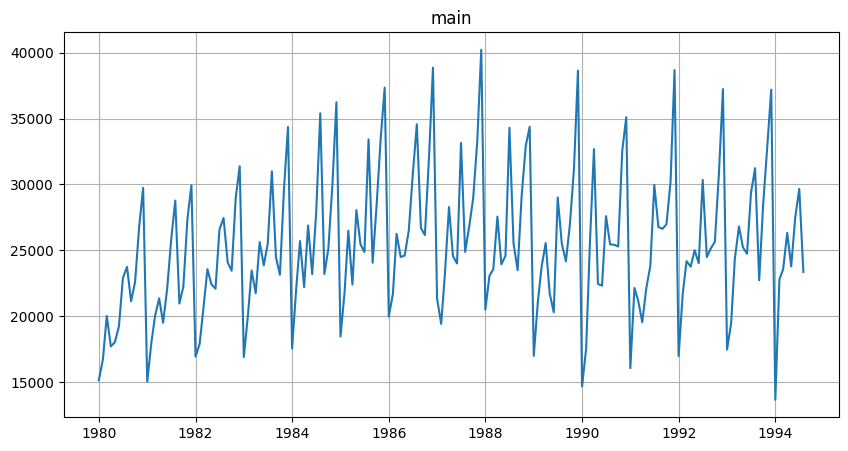
Let’s load and look at the dataset
[2]:
import pandas as pd
[3]:
original_df = pd.read_csv("data/monthly-australian-wine-sales.csv")
original_df.head()
[3]:
| month | sales | |
|---|---|---|
| 0 | 1980-01-01 | 15136 |
| 1 | 1980-02-01 | 16733 |
| 2 | 1980-03-01 | 20016 |
| 3 | 1980-04-01 | 17708 |
| 4 | 1980-05-01 | 18019 |
etna_ts is strict about data format: * column we want to predict should be called target * column with datatime data should be called timestamp * because etna is always ready to work with multiple time series, column segment is also compulsory
Our library works with the special data structure TSDataset. So, before starting anything, we need to convert the classical DataFrame to TSDataset.
Let’s rename first
[4]:
original_df["timestamp"] = pd.to_datetime(original_df["month"])
original_df["target"] = original_df["sales"]
original_df.drop(columns=["month", "sales"], inplace=True)
original_df["segment"] = "main"
original_df.head()
[4]:
| timestamp | target | segment | |
|---|---|---|---|
| 0 | 1980-01-01 | 15136 | main |
| 1 | 1980-02-01 | 16733 | main |
| 2 | 1980-03-01 | 20016 | main |
| 3 | 1980-04-01 | 17708 | main |
| 4 | 1980-05-01 | 18019 | main |
Time to convert to TSDataset!
To do this, we initially need to convert the classical DataFrame to the special format.
[5]:
from etna.datasets.tsdataset import TSDataset
[6]:
df = TSDataset.to_dataset(original_df)
df.head()
[6]:
| segment | main |
|---|---|
| feature | target |
| timestamp | |
| 1980-01-01 | 15136 |
| 1980-02-01 | 16733 |
| 1980-03-01 | 20016 |
| 1980-04-01 | 17708 |
| 1980-05-01 | 18019 |
Now we can construct the TSDataset.
Additionally to passing dataframe we should specify frequency of our data. In this case it is monthly data.
[7]:
ts = TSDataset(df, freq="1M")
/Users/a.p.chikov/PycharmProjects/etna_dev/etna-ts/etna/datasets/tsdataset.py:144: UserWarning: You probably set wrong freq. Discovered freq in you data is MS, you set 1M
  warnings.warn(
Oups. Let’s fix that
[8]:
ts = TSDataset(df, freq="MS")
We can look at the basic information about the dataset
[9]:
ts.info()
<class 'etna.datasets.TSDataset'>
num_segments: 1
num_exogs: 0
num_regressors: 0
num_known_future: 0
freq: MS
         start_timestamp end_timestamp  length  num_missing
segments
main          1980-01-01    1994-08-01     176            0
Or in DataFrame format
[10]:
ts.describe()
[10]:
| start_timestamp | end_timestamp | length | num_missing | num_segments | num_exogs | num_regressors | num_known_future | freq | |
|---|---|---|---|---|---|---|---|---|---|
| segments | |||||||||
| main | 1980-01-01 | 1994-08-01 | 176 | 0 | 1 | 0 | 0 | 0 | MS |
3. Forecasting single time series
Our library contains a wide range of different models for time series forecasting. Let’s look at some of them.
3.1 Simple forecast
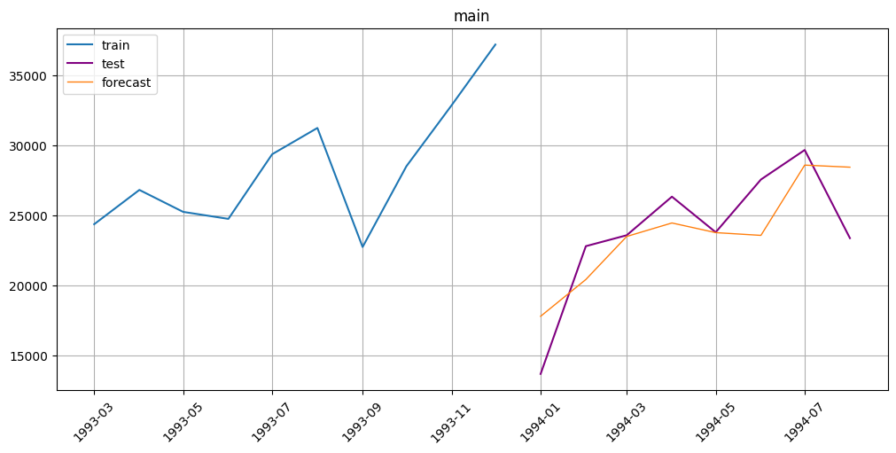
Let’s predict the monthly values in 1994 in our dataset using the NaiveModel
[12]:
train_ts, test_ts = ts.train_test_split(
    train_start="1980-01-01",
    train_end="1993-12-01",
    test_start="1994-01-01",
    test_end="1994-08-01",
)
[13]:
HORIZON = 8
from etna.models import NaiveModel

# Fit the model
model = NaiveModel(lag=12)
model.fit(train_ts)

# Make the forecast
future_ts = train_ts.make_future(future_steps=HORIZON, tail_steps=model.context_size)
forecast_ts = model.forecast(future_ts, prediction_size=HORIZON)
Here we pass prediction_size parameter during forecast because in forecast_ts few first points are dedicated to be a context for NaiveModel.
Now let’s look at a metric and plot the prediction. All the methods already built-in in etna.
[14]:
from etna.metrics import SMAPE
[15]:
smape = SMAPE()
smape(y_true=test_ts, y_pred=forecast_ts)
[15]:
{'main': 11.492045838249387}
[16]:
from etna.analysis import plot_forecast
[17]:
plot_forecast(forecast_ts, test_ts, train_ts, n_train_samples=10)

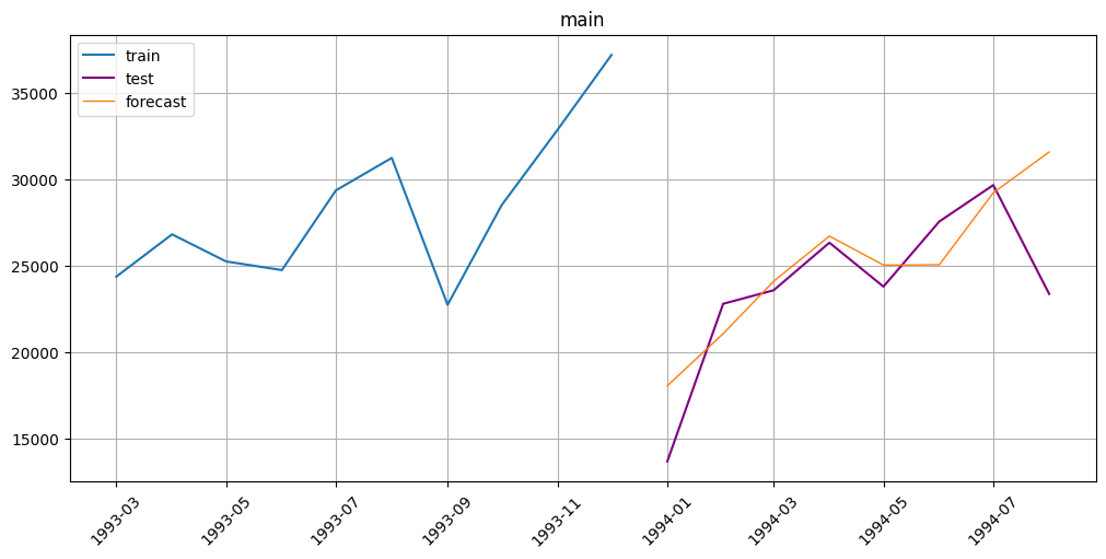
3.2 Prophet
Now try to improve the forecast and predict the values with Prophet.
[18]:
from etna.models import ProphetModel

model = ProphetModel()
model.fit(train_ts)

# Make the forecast
future_ts = train_ts.make_future(HORIZON)
forecast_ts = model.forecast(future_ts)
10:12:40 - cmdstanpy - INFO - Chain [1] start processing
10:12:40 - cmdstanpy - INFO - Chain [1] done processing
[19]:
smape(y_true=test_ts, y_pred=forecast_ts)
[19]:
{'main': 10.510260655718435}
[20]:
plot_forecast(forecast_ts, test_ts, train_ts, n_train_samples=10)
3.2 Catboost
And finally let’s try the Catboost model.
Also etna has wide range of transforms you may apply to your data.
Transforms are not stored in the dataset, so you should pass them explicitly to transform, inverse_transform and make_future methods.
Here how it is done:
[21]:
from etna.transforms import LagTransform, LogTransform

lags = LagTransform(in_column="target", lags=list(range(8, 24, 1)))
log = LogTransform(in_column="target")
transforms = [log, lags]
train_ts.fit_transform(transforms)
[22]:
from etna.models import CatBoostMultiSegmentModel

model = CatBoostMultiSegmentModel()
model.fit(train_ts)
future_ts = train_ts.make_future(future_steps=HORIZON, transforms=transforms)
forecast_ts = model.forecast(future_ts)
forecast_ts.inverse_transform(transforms)
[23]:
from etna.metrics import SMAPE

smape = SMAPE()
smape(y_true=test_ts, y_pred=forecast_ts)
[23]:
{'main': 10.657026308972483}
[24]:
from etna.analysis import plot_forecast

train_ts.inverse_transform(transforms)
plot_forecast(forecast_ts, test_ts, train_ts, n_train_samples=10)
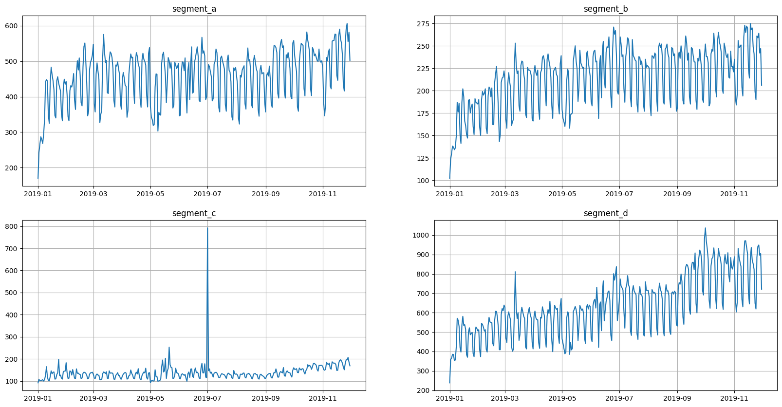
4. Forecasting multiple time series
In this section you may see example of how easily etna works with multiple time series and get acquainted with other transforms etna contains.
[25]:
original_df = pd.read_csv("data/example_dataset.csv")
original_df.head()
[25]:
| timestamp | segment | target | |
|---|---|---|---|
| 0 | 2019-01-01 | segment_a | 170 |
| 1 | 2019-01-02 | segment_a | 243 |
| 2 | 2019-01-03 | segment_a | 267 |
| 3 | 2019-01-04 | segment_a | 287 |
| 4 | 2019-01-05 | segment_a | 279 |
[26]:
df = TSDataset.to_dataset(original_df)
ts = TSDataset(df, freq="D")
ts.plot()
[27]:
ts.info()
<class 'etna.datasets.TSDataset'>
num_segments: 4
num_exogs: 0
num_regressors: 0
num_known_future: 0
freq: D
          start_timestamp end_timestamp  length  num_missing
segments
segment_a      2019-01-01    2019-11-30     334            0
segment_b      2019-01-01    2019-11-30     334            0
segment_c      2019-01-01    2019-11-30     334            0
segment_d      2019-01-01    2019-11-30     334            0
[28]:
import warnings

from etna.transforms import (
    MeanTransform,
    LagTransform,
    LogTransform,
    SegmentEncoderTransform,
    DateFlagsTransform,
    LinearTrendTransform,
)

warnings.filterwarnings("ignore")

log = LogTransform(in_column="target")
trend = LinearTrendTransform(in_column="target")
seg = SegmentEncoderTransform()

lags = LagTransform(in_column="target", lags=list(range(30, 96, 1)))
d_flags = DateFlagsTransform(
    day_number_in_week=True,
    day_number_in_month=True,
    week_number_in_month=True,
    week_number_in_year=True,
    month_number_in_year=True,
    year_number=True,
    special_days_in_week=[5, 6],
)
mean30 = MeanTransform(in_column="target", window=30)
transforms = [log, trend, lags, d_flags, seg, mean30]
[29]:
HORIZON = 30
train_ts, test_ts = ts.train_test_split(
    train_start="2019-01-01",
    train_end="2019-10-31",
    test_start="2019-11-01",
    test_end="2019-11-30",
)
train_ts.fit_transform(transforms)
[30]:
test_ts.info()
<class 'etna.datasets.TSDataset'>
num_segments: 4
num_exogs: 0
num_regressors: 0
num_known_future: 0
freq: D
          start_timestamp end_timestamp  length  num_missing
segments
segment_a      2019-11-01    2019-11-30      30            0
segment_b      2019-11-01    2019-11-30      30            0
segment_c      2019-11-01    2019-11-30      30            0
segment_d      2019-11-01    2019-11-30      30            0
[31]:
from etna.models.catboost import CatBoostMultiSegmentModel

model = CatBoostMultiSegmentModel()
model.fit(train_ts)
future_ts = train_ts.make_future(future_steps=HORIZON, transforms=transforms)
forecast_ts = model.forecast(future_ts)
forecast_ts.inverse_transform(transforms)
[32]:
smape = SMAPE()
smape(y_true=test_ts, y_pred=forecast_ts)
[32]:
{'segment_d': 4.98784059255331,
 'segment_c': 11.729007773459314,
 'segment_b': 4.210896545479218,
 'segment_a': 6.059390208724575}
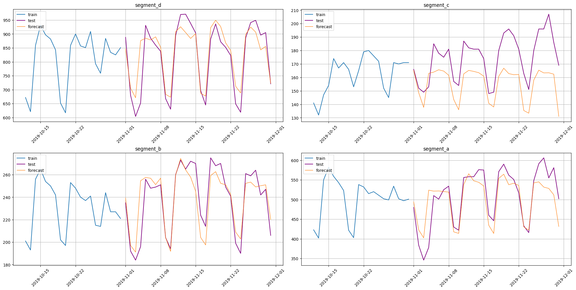
[33]:
train_ts.inverse_transform(transforms)
plot_forecast(forecast_ts, test_ts, train_ts, n_train_samples=20)
5. Pipeline
Let’s wrap everything into pipeline to create the end-to-end model from previous section.
[34]:
from etna.pipeline import Pipeline
[35]:
train_ts, test_ts = ts.train_test_split(
    train_start="2019-01-01",
    train_end="2019-10-31",
    test_start="2019-11-01",
    test_end="2019-11-30",
)
We put: model, transforms and horizon in a single object, which has the similar interface with the model(fit/forecast)
[36]:
model = Pipeline(
    model=CatBoostMultiSegmentModel(),
    transforms=transforms,
    horizon=HORIZON,
)
model.fit(train_ts)
forecast_ts = model.forecast()
As in the previous section, let’s calculate the metrics and plot the forecast
[37]:
smape = SMAPE()
smape(y_true=test_ts, y_pred=forecast_ts)
[37]:
{'segment_d': 4.98784059255331,
 'segment_c': 11.729007773459314,
 'segment_b': 4.210896545479218,
 'segment_a': 6.059390208724575}
[38]:
plot_forecast(forecast_ts, test_ts, train_ts, n_train_samples=20)
