Outliers notebook
![]()
This notebook contains the simple examples of outliers handling using ETNA library.
Table of Contents
[1]:
import warnings

warnings.filterwarnings("ignore")
1. Uploading dataset
[2]:
import pandas as pd
from etna.datasets.tsdataset import TSDataset
Let’s load and look at the dataset
[3]:
classic_df = pd.read_csv("data/example_dataset.csv")
df = TSDataset.to_dataset(classic_df)
ts = TSDataset(df, freq="D")
ts.head(5)
[3]:
| segment | segment_a | segment_b | segment_c | segment_d |
|---|---|---|---|---|
| feature | target | target | target | target |
| timestamp | ||||
| 2019-01-01 | 170 | 102 | 92 | 238 |
| 2019-01-02 | 243 | 123 | 107 | 358 |
| 2019-01-03 | 267 | 130 | 103 | 366 |
| 2019-01-04 | 287 | 138 | 103 | 385 |
| 2019-01-05 | 279 | 137 | 104 | 384 |
As you can see from the plots, all the time series contain outliers - abnormal spikes on the plot.
[4]:
ts.plot()
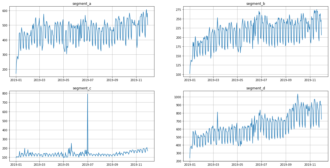
In our library, we provide methods for point outliers detection, visualization and imputation. In the sections below, you will find an overview of the outliers handling tools.
2. Point outliers
Point outliers are stand alone abnormal spikes on the plot. Our library contains four methods for their detection based on different principles. The choice of the method depends on the dataset.
[5]:
from etna.analysis import (
    get_anomalies_median,
    get_anomalies_density,
    get_anomalies_prediction_interval,
    get_anomalies_hist,
)
from etna.analysis import plot_anomalies
Note: you can specify the column in which you want search for anomalies using the in_column argument.
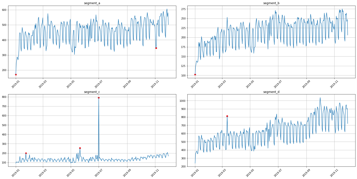
3.1 Median method
To obtain the point outliers using the median method we need to specify the window for fitting the median model.
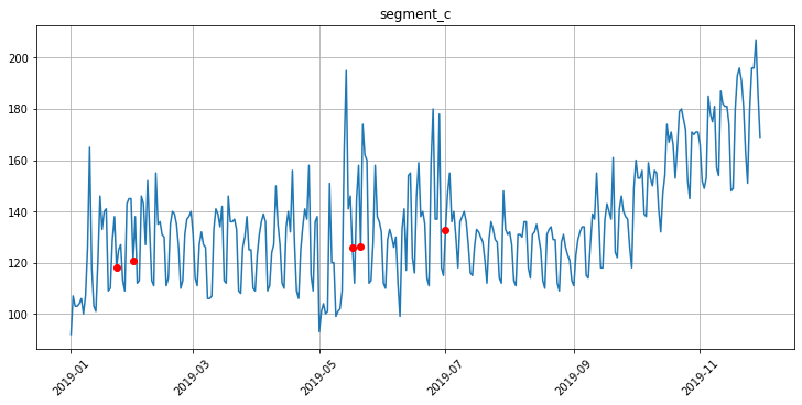
[6]:
anomaly_dict = get_anomalies_median(ts, window_size=100)
plot_anomalies(ts, anomaly_dict)

3.2 Density method
It is a distance-based method for outliers detection.
[7]:
anomaly_dict = get_anomalies_density(ts, window_size=18, distance_coef=1, n_neighbors=4)
plot_anomalies(ts, anomaly_dict)
3.3 Prediction interval method
It is a model-based method for outliers detection. Outliers here are all points out of the prediction interval predicted with the model.
Note: method is now available only for ProphetModel and SARIMAXModel.
[8]:
from etna.models import ProphetModel
[9]:
anomaly_dict = get_anomalies_prediction_interval(ts, model=ProphetModel, interval_width=0.95)
plot_anomalies(ts, anomaly_dict)
12:33:49 - cmdstanpy - INFO - Chain [1] start processing
12:33:49 - cmdstanpy - INFO - Chain [1] done processing
12:33:49 - cmdstanpy - INFO - Chain [1] start processing
12:33:49 - cmdstanpy - INFO - Chain [1] done processing
12:33:49 - cmdstanpy - INFO - Chain [1] start processing
12:33:49 - cmdstanpy - INFO - Chain [1] done processing
12:33:49 - cmdstanpy - INFO - Chain [1] start processing
12:33:50 - cmdstanpy - INFO - Chain [1] done processing

3.4 Histogram method
This method detects outliers in time series using histogram model. Outliers here are all points that, when removed, result in a histogram with a lower approximation error.
Note: method might work sufficiently slow.
[10]:
anomaly_dict = get_anomalies_hist(ts, bins_number=10)
plot_anomalies(ts, anomaly_dict)

3. Interactive visualization
The performance of outliers detection methods significantly depends on their hyperparameters values. To select the best parameters’ configuration for the chosen method, you can use our interactive visualization tool.
[11]:
from etna.analysis import plot_anomalies_interactive
You only need to specify segment, the outliers detection method and it’s parameters grid in format (min, max, step) for each parameter you want to control.
[12]:
segment = "segment_c"
method = get_anomalies_median
params_bounds = {"window_size": (40, 70, 1), "alpha": (0.1, 4, 0.25)}
In some cases there might be troubles with this visualisation in Jupyter notebook, try to use !jupyter nbextension enable --py widgetsnbextension
[13]:
plot_anomalies_interactive(ts=ts, segment=segment, method=method, params_bounds=params_bounds)
Let’s assume that the best parameters are:
[14]:
best_params = {"window_size": 60, "alpha": 2.35}
4. Outliers imputation
The previous sections are focused on the outliers detection as the part of the EDA, however outliers imputation might be also one of the step in the pipeline of your forecasting model. Let’s explore a simple example of how to build such pipeline.
[15]:
from etna.transforms import MedianOutliersTransform, TimeSeriesImputerTransform
from etna.analysis import plot_imputation
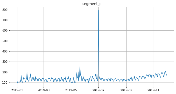
Segment with outliers:
[16]:
df = ts[:, segment, :]
ts = TSDataset(df, freq="D")
ts.plot()
Outliers imputation process consists of two steps: 1. Replace the outliers, detected by the specific method, with NaNs using the instance of the corresponding OutliersTransform
Impute NaNs using the TimeSeriesImputerTransform
Before the imputation step you firstly need to choose the appropriate imputation method and you can do it using our EDA method for imputation visualisation - plot_imputation.
[17]:
# Impute outliers with NaNs
outliers_remover = MedianOutliersTransform(in_column="target", **best_params)

ts.fit_transform([outliers_remover])
ts.plot()
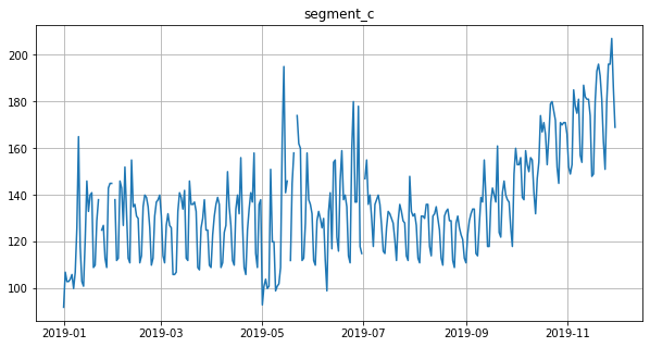
Let’s impute outliers detected by median method using the running_mean imputation strategy.
[18]:
# Impute NaNs using the specified strategy
outliers_imputer = TimeSeriesImputerTransform(in_column="target", strategy="running_mean", window=30)
Let’s look at the points that we replaced with TimeSeriesImputerTransform using plot_imputation.
[19]:
plot_imputation(imputer=outliers_imputer, ts=ts)
[20]:
ts.fit_transform([outliers_imputer])
Now you can fit the model on the cleaned dataset, which might improve the forecasting quality. Let’s compare the forecasts of the model fitted on cleaned and uncleaned train timeseries.
[21]:
from etna.models import MovingAverageModel
from etna.pipeline import Pipeline
from etna.metrics import MAE, MSE, SMAPE
[22]:
def get_metrics(forecast, test):
    """Compute the metrics on forecast"""
    metrics = {"MAE": MAE(), "MSE": MSE(), "SMAPE": SMAPE()}
    results = dict()
    for name, metric in metrics.items():
        results[name] = metric(y_true=test, y_pred=forecast)["segment_c"]
    return results
[23]:
def test_transforms(transforms=[]):
    """Run the experiment on the list of transforms"""
    classic_df = pd.read_csv("data/example_dataset.csv")
    df = TSDataset.to_dataset(classic_df[classic_df["segment"] == segment])
    ts = TSDataset(df, freq="D")
    train, test = ts.train_test_split(
        train_start="2019-05-20",
        train_end="2019-07-10",
        test_start="2019-07-11",
        test_end="2019-08-09",
    )

    model = Pipeline(model=MovingAverageModel(window=30), transforms=transforms, horizon=30)
    model.fit(train)
    forecast = model.forecast()
    metrics = get_metrics(forecast, test)
    return metrics
Results on the uncleaned dataset:
[24]:
test_transforms()
[24]:
{'MAE': 40.08799715116714,
 'MSE': 1704.8554888537708,
 'SMAPE': 27.36913416466395}
Results on the cleaned dataset(we impute outliers in train part and predict the test part):
[25]:
transforms = [outliers_remover, outliers_imputer]
test_transforms(transforms)
[25]:
{'MAE': 11.606826505006092,
 'MSE': 196.5736131226554,
 'SMAPE': 8.94919204071121}
As you can see, there is significant improvement in the metrics in our case. However, the points that we defined as the outliers may occur to be the points of complex timeseries behavior. In this case, outliers imputation might make the forecast worse.